Dreamer
Introduction
Dreamer learns a compact simulator from experience and trains a policy inside that simulator. The world model predicts the consequences of actions, the critic estimates future return from the resulting states, and the actor learns to choose actions that increase expected return. Training the actor and critic primarily on imagined trajectories can improve sample efficiency by reducing the amount of real environment interaction needed to learn a useful policy.
Although intuitively appealing, authors note that robustly learning and leveraging world models to achieve strong task performance has been an open problem and required a range of robustness techniques based on normalization, balancing, and transformations.
The three networks - the dynamics model, the critic, and the actor - are trained concurrently from replayed experience while the agent interacts with the environment. Authors note that in order to succeed across domains, all three components need to accomodate different signal magnitudes and robustly balance terms in their objectives; this is challenging because they want to achieve robust performance across diverse domains with fixed hyperparameters.
For Dreamer V3, which we focus on in this note, the world model is implemented as a Recurrent State-Space Model (RSSM). An encoder maps sensory inputs to stochastic representations . Then, a sequence model with recurrent state predicts the sequence of these representations given past actions .
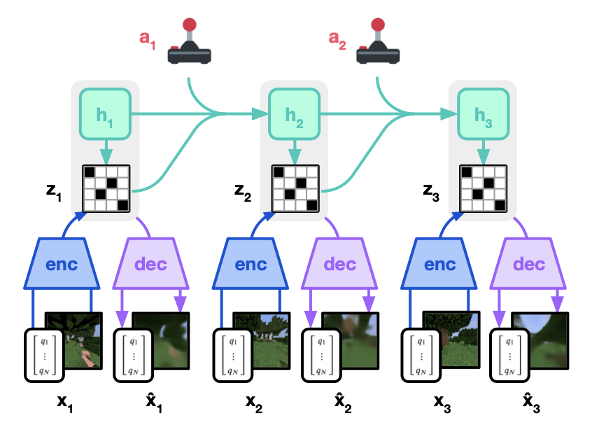
The model state is the concatenation of a deterministic recurrent state and a stochastic representation . summarizes the past but cannot express uncertainty, while is a compact code of the current observation. The encoder gives a posterior that captures the new information in the observation, and the dynamics predictor gives a prior over possible next states.
Before Dreamer V1-V4, PlaNet used online trajectory optimization with a Gaussian RSSM. Dreamer V1 also used a Gaussian RSSM, Dreamer V2 and V3 used a categorical RSSM, and Dreamer V4 uses a transformer. Broadly, model learning learns to predict which observations and rewards are plausible given an action and observation history. Behaviour learning, meanwhile, learns which actions produce high return under a learned model. The two, while similar, have different problems - a model can predict well but yield a policy that chooses ineffective actions, while behaviour policies can learn to exploit errors in the model that don’t transfer into the real world. Unlike PlaNet, Dreamer consolidates the cost of trajectory optimization into a single network forward pass.
We use the following convention throughout: at time , the agent sees , has just received reward from action , forms a model state , and chooses . The environment then returns . Here means the transition terminates the task; otherwise it is 1. This convention makes formulating the training problem for a reward head on natural.
| Symbol | Meaning |
|---|---|
| Observation, outgoing action, arriving reward, continuation label. | |
| Deterministic memory, stochastic latent, full RSSM state . | |
| Observation-informed posterior (recognition model). | |
| Predictive prior, available without the current observation. | |
| World-model, actor, and critic parameters. | |
| Action distribution and expected future return. | |
| Discount factor, return mixing coefficient, imagination horizon. | |
| Same forward value as , but zero derivative through this occurrence. | |
| Replay batch size, sequence length, latent factors, classes per factor. |
The objective of a policy is expected discounted reward:
Training of Dreamer has two connected components:
- Fit the world model to recorded trajectories
- Use multi-step trajectories to train the actor and the critic.
Let’s delve into both. In this note, we specifically focus on Dreamer V3.

Training the World Model
Dreamer V1-V3 used a Recurrent State Space Model (RSSM) for its world model, a recurrent network architecture that is able to both capture representations of observation and action history along with a multimodal belief over the current state.
The RSSM’s state is composed of , which represents an encoding of the action and observation history, along with , a latent sample of a learned representation of the posterior . The observation encoder is denoted .
Training occurs in the following steps. First, sample a real trajectory from replay. The observations, actions, rewards, and continuation labels in this part were actually recorded from the environment:
-
Propogate memory:
-
Compute the posterior:
The full state is now . We evaluate the world model losses here, at the observation-informed state. The observation decoder is compared against the recorded , the reward head against the recorded , and the continuation head against the recorded . The prior is also compared with the posterior distribution through the KL losses.
I go over a numerical example of how to conduct forward passes and backpropogation through the categorical sampling of the latent in the Appendix.
-
Propogate memory:
Here is the next recorded action. Repeat over the sequence and aggregate the losses to update the world-model parameters .
The observation therefore reaches deterministic memory along the path
The posterior network is trained partly through the observation decoder, which reconstructs the observation from the latent state . The reconstruction loss compares this prediction with the actual observation, and its gradients update both the decoder and the posterior network. Meanwhile, the prior is trained to match the observation-informed posterior . The posterior is also regularized toward the prior, encouraging a representation that remains informative about the observation while being predictable from history and actions.
The prediction losses have the form
Each here denotes the relevant output head, rather than the latent prior. In V3, reward prediction uses a two-hot cross-entropy target, continuation uses binary cross-entropy, and observation reconstruction uses the loss appropriate to the input modality.
Writing and , the two KL branches are
These two terms are constructed because of the following:
- The allows for some disagreement between the prior and posterior without a penalty gradient, since the posterior learning more accurate outcomes also benefits the actor and critic training.
- While we could have a single term , keeping them separate permits the objective to weigh divergence between the two learned distributions separately, putting more pressure on the prior to match the posterior than vice versa.
The world-model loss then averages over replay batch and time.
Training the Actor and Critic
Imagination lets Dreamer learn from simulated experience, reducing the need for real environment interactions and therefore improving sample efficiency. The actor learns which actions to take while the critic estimates the future return from a state when following that actor. These updates alternate with world-model training throughout learning, but the world model is fixed during each behaviour (actor+critic) update. The losses below follow Dreamer V3.
-
Generate an imagined trajectory
We start from an observation-informed state inferred from real replay, detach it from the world-model training graph, and call it . Here, a hat indicates an imagined quantity (similar to state estimate in controls), counts imagination steps, and is the rollout horizon. The different indices may be confusing, but what we’re saying is to take the state at real trajectory time , and use it as the starting state of imagination.
At each step, the actor samples an action and the world model predicts its consequence:
There is no new observation from the true environment here, so the latent comes from the prior (this is what we train the prior for). At , the reward head predicts the arriving reward and the continuation head predicts the probability that the episode continues. Repeat for transitions:
The critic evaluates each state, producing for . Each value estimates future return, and the final state is the one where imagination stops.
-
Forming the return target
The critic is trained by bootstrapping. We need a training target estimating how much discounted reward follows each state. Beyond the rollout, we use the critic’s estimate:
Then we work backward, from to :
Going term by term:
- is the predicted reward from the next transition.
- discounts rewards further into the future; gates the future contribution by continuation probability.
- estimates the remaining return directly from the next state.
- uses more of the imagined trajectory. The mixing parameter balances these two estimates.
With , the target uses one predicted reward and the next critic value. With , it uses all remaining imagined rewards and the final critic value. Intermediate choices give -returns, and Dreamer V3 uses by default. This means the training target mixes 5% of the critic value with 95% of the return target, which relies on the critic at the terminal state of the imagination and largely on the world model’s reward head before the terminal state.
-
Training the critic
The basic task is to bring closer to . Conceptually, a squared-error critic would minimize .
V3 instead predicts a probability distribution over fixed, exponentially spaced return bins . Its scalar value is the probability-weighted mean:
Convert the target into : place weight on the two neighboring bins, with more weight on the closer one. For example, a target of 3 between bins 2 and 6 gets weights and .
Later imagined states receive less weight if they are unlikely to be reached before termination. Define discounted continuation weights
The main critic loss is the cross-entropy between the target bin weights and predicted probabilities:
Here indexes bins, indexes rollout steps, and denotes averaging over sampled starting states and rollouts. Minimizing this loss puts more predicted probability on bins supported by the return target.
You may ask - why do we need probability bins over training on the target directly? That’s a good question. Recall that Dreamer is intended to be easily ported to new domains, and different domains may have drastically different return magnitudes. By using binning, we make the training less sensitive to reward magnitudes.
V3 also stabilizes the critic with a penalty toward a slowly averaged critic’s predictions and an auxiliary replay-value loss, weighted by . The latter combines real replay rewards with imagined return estimates at replay states, but the equation above shows the main imagination loss.
-
Training the actor
The advantage of an action taken by the actor is the return from the taken action minus the value of being in the origin state as estimated by the critic:
If and , the sampled action has advantage : its sampled imagined outcome was better than the baseline.
To control update scale, define
where is an exponentially smoothed estimate of the 95th-minus-5th percentile range of imagined returns. The denominator scales down large advantages without amplifying small ones.
The actor loss is
The sampled actions and states are treated as fixed inputs in this V3 update. The terms mean:
- is the log probability (or log density for continuous actions) the actor assigns to the sampled action. With the leading minus sign, minimizing the loss increases it for positive advantages and decreases it for negative ones.
- is the policy’s entropy. Its positive coefficient inside the brackets rewards maintaining exploration.
- is the same discounted continuation weight used above.
Inference
After training, the agent receives real observations during execution and uses the posterior. The observation encoder is used during deployment too. With the learned parameters fixed, each step is:
-
Receive and update memory using the previous inferred state and the action actually taken:
-
Encode the observation and infer the current latent:
-
Choose an action with the actor:
-
Execute in the environment. Receive , , and ; carry into the next step. At a new episode, reset the recurrent carry and previous-action input according to the implementation.
The observation encoder and posterior remain active during real-world execution because fresh observations are available. The observation decoder, reward predictor, and critic are not used during inference.
Appendix
-
How do we get gradients through categorical sampling in the RSSM?
A categorical sample from the categorical representation of the posterior is discrete. Ordinary backpropagation cannot differentiate through the choice of category. DreamerV3 uses a straight-through estimator, where the forward pass uses a sampled one-hot vector, while the backward pass follows the probabilities that generated it. This lets reconstruction and other prediction losses train the posterior through its sampled latent. Let’s work through an example to see how it works.
Consider one three-category factor in the posterior. Let its logits be , with probabilities
Here denotes this probability vector (note this example omits V3’s 1% uniform mixing). Suppose sampling selects category 2:
Construct the latent passed to the decoder as
Forward pass. Stop-gradient does not change numerical values, so
The observation decoder then sees this sample, and losses are evaluated relative to it.
Backward pass. The stopped term contributes no derivative, leaving
Thus the downstream gradient passes unchanged from to , then passes through the softmax to the logits. The forward value is hard, but the backward path is differentiable.
For a concrete reconstruction example, use a toy scalar decoder
Treat as a column vector here. Our sample gives and . The decoder sends back
The straight-through rule gives the same gradient . Using the softmax derivative,
Since , the logit gradient is
Gradient descent subtracts this gradient, lowering the first two logits and raises the third. In this toy example, the backward signal pushes toward a higher decoder output. That signal then propagates into the posterior network’s parameters and the decoder also receives its own parameter gradients.
In PyTorch, this looks like:
probs = logits.softmax(dim=-1)
sample = torch.distributions.OneHotCategorical(probs=probs).sample()
z = probs + (sample - probs).detach()
Note that this is a biased gradient approximation, and not the exact derivative of categorical sampling or a guarantee that every update improves the expected loss. The numerical gradient above is the surrogate gradient chosen by the estimator. The prior–posterior KL loss compares distributions directly, so it does not need this estimator to differentiate through a sample.